Abstract
This post delves into the implementation of my procedural earth simulation, written entirely in GLSL fragment shaders. It simulates the complete history of an earth-like planet in a few minutes, with the simulation updating at 60 frames per second.
Protoplanet
This story begins four and a half billion years ago, with a lump of molten rock...
The early earth was a protoplanet, red hot and heavily cratered by asteroid impacts. As my earth simulation is entirely procedurally generated, with no pre-rendered textures, the first task is to generate a map of this terrain. To calculate the height of the terrain at a given latitude and longitude, first translate to 3D cartesian coordinates:
vec3 p = 1.5 * vec3(
    sin(lon*PI/180.) * cos(lat*PI/180.),
    sin(lat*PI/180.),
    cos(lon*PI/180.) * cos(lat*PI/180.));
Now, as asteroids come in a variety of sizes, so do the resulting craters. To accommodate this, the shader iterates over five levels of detail, layering craters of decreasing size over each other. To make the craters have a realistic rugged appearance, this is mixed with some fractional Brownian motion noise, and scaled so that the largest craters have the most impact on the terrain.
float height = 0.;
for (float i = 0.; i < 5.; i++) {
    float c = craters(0.4 * pow(2.2, i) * p);
    float noise = 0.4 * exp(-3. * c) * FBM(10. * p);
    float w = clamp(3. * pow(0.4, i), 0., 1.);
    height += w * (c + noise);
}
height = pow(height, 3.);
The craters themselves are generated on a 3D grid, from which a sphere is carved out for the surface terrain. To avoid visible regularity, the crater centres are given a pseudo-random offset from the grid points, using a hash function. To calculate influence of a crater at a given location, take a weighted average of the craters belonging to the nearby grid points, with weights exponentially decreasing with distance from the centre. The crater rims are generated by a simple sine curve.
float craters(vec3 x) {
    vec3 p = floor(x);
    vec3 f = fract(x);
    float va = 0.;
    float wt = 0.;
    for (int i = -2; i <= 2; i++)
     for (int j = -2; j <= 2; j++)
      for (int k = -2; k <= 2; k++) {
        vec3 g = vec3(i,j,k);
        vec3 o = 0.8 * hash33(p + g);
        float d = distance(f - g, o);
        float w = exp(-4. * d);
        va += w * sin(2.*PI * sqrt(d));
        wt += w;
    }
    return abs(va / wt);
}
The final procedurally generated heightmap looks like this:
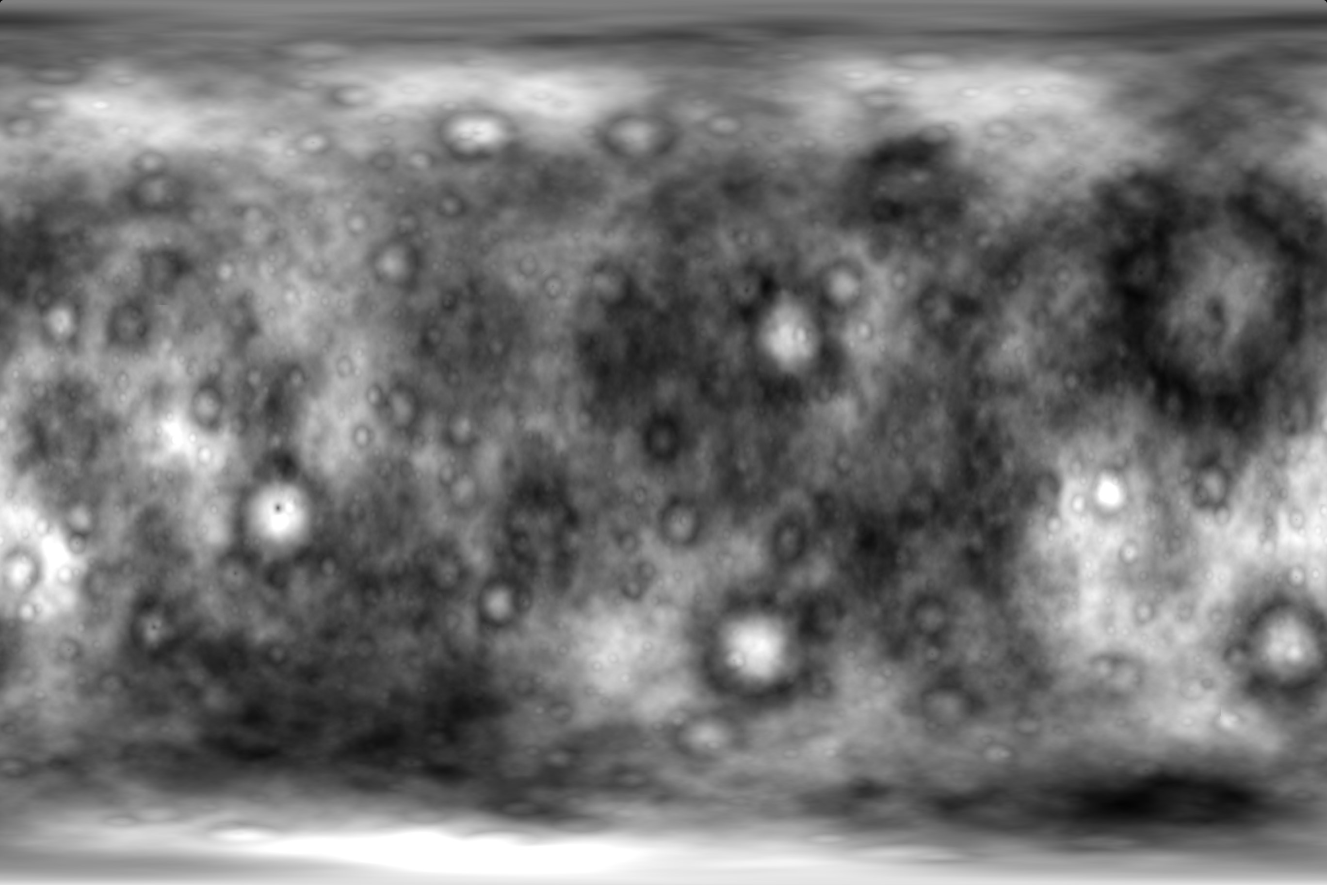
Although relatively simple, after filling the low-lying regions with water, this procedural terrain resembles what scientists believe the early earth actually looked like:
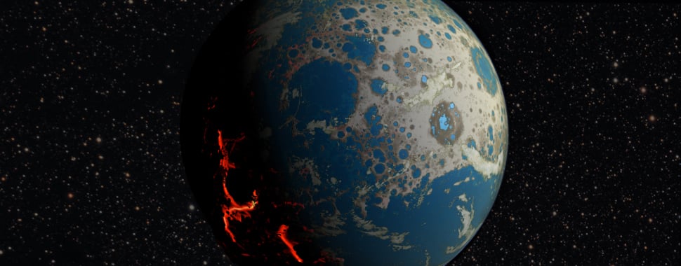
Water contained within was vaporised by the heat, which escaped and began circulating through the early atmosphere forming around the planet. As time progressed and the rock cooled, the water vapour began to condense into oceans. The flow of liquid water across the surface carved valleys in the terrain, leaving an accumulation of sediment in its wake.
Tectonic plates
The formation of mountains, ocean trenches, and familiar continental landforms requires a model of tectonic movement. The simulation randomly generates seed locations for plates, with an initial velocity. These plates grow in size over time with a simple aggregation model, which randomly selects neighbouring points and adds them to a plate if they have not already been assigned to another plate. All of the pixels within a plate store the velocity of the plate's movement. The aggregation model is similar to that of a diffusion-limited aggregation (but without the diffusion):
Continuous movement of the plates is difficult, as it would require plate boundaries to account for movements measured in fractions of a pixel. To avoid this, the plates are instead moved at discrete time-steps, by a whole pixel either horizontally or vertically. These times are randomised for each plate such that the average velocity is maintained at the set speed and direction, and also so that it is unlikely that neighbouring plates will move simultaneously.
Plate collisions occur when some boundary pixels of one plate move onto a location previously occupied by pixels belonging to another plate. This causes subduction, which is modelled by simply slightly increasing the elevation of the terrain at the locations of the collision. Although this only occurs at the pixels along the boundary of a plate, the impact is gradually spread to neighbouring pixels through a simple thermal erosion model, which pushes the elevation of a pixel in the direction of the average of its neighbours.
Altogether this provides a decent simulation of the formation of continents with mountain ranges (which will be further improved with the introduction of hydraulic erosion in the next section):
Hydraulic erosion
The rugged appearance of natural terrain is largely driven by the formation of river basins, which erode landscapes in a familiar branching pattern. A variety of water flow simulations are readily available for this task, but a difficulty here is that the resolution of the terrain map is quite low for an entire planet. Therefore, the model will have to be able to simulate rivers which are no more than a single pixel wide. Barnes (2018) proposes a simple model which achieves just this.
Simply put, each pixel examines its eight neighbours, to determine which direction has the greatest decrease in elevation (adjusted for the fact that the diagonal neighbours are further away). This direction of greatest slope is where water flowing out of this pixel will travel. Water is initially distributed amongst cells by rainfall, which is then transported between neighbouring pixels at each time-step.
Erosion is driven by a stream power law:
elevation -= 0.05 * pow(water, 0.8) * pow(slope, 2.);
Here we have the elevation and amount of water located at the current cell, along with the slope in the direction the water is travelling. The decrease in elevation is capped so that it doesn't become lower than the location the water is flowing to.
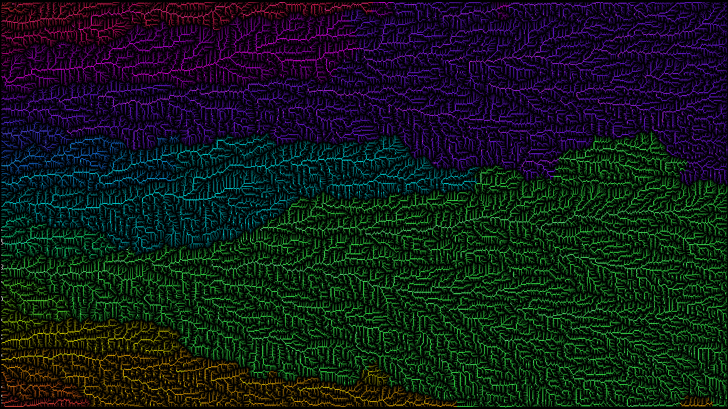
The interaction between the water flow and erosion results in the natural formation of river basins in the terrain:
By colouring connected waterways (with the colour determined by the location of the river's mouth), it's possible to produce striking visualisations reminiscent of real river basin maps:

Global climate
Simulating the climate system of an entire planet is a daunting task, but luckily it turns out that it can be approximated relatively easily. The driving force behind everything in my climate simulation is a procedurally generated map of the mean sea-level pressure (MSLP).
According to the Climate Cookbook, the main ingredients in creating a MSLP map are where the landforms are located amidst the ocean, and the impact of latitude. In fact, if you take data from a real MSLP map of the Earth, separate out locations according to whether they are land or ocean, and plot the MSLP against latitude, you end up with two sinusoidal curves for the land and ocean with slightly different shapes.
By fitting the parameters appropriately, I came up with a crude model of the annual mean pressure (here the latitude is measured in degrees):
if (land) {
    mslp = 1012.5 - 6. * cos(lat*PI/45.);
} else { // ocean
    mslp = 1014.5 - 20. * cos(lat*PI/30.);
}
Of course, this isn't quite enough to generate a realistic MSLP map, as generating values for the land and ocean separately results in sharp discontinuities at the boundaries between them. In reality, MSLP smoothly varies across the transition from ocean to land, due to the local diffusion of gas pressure. This diffusion process can be approximated quite well by simply applying a Gaussian blur to the MSLP map (with a standard deviation of 10--15 degrees).
To allow for the climate to change along with the seasons, it's necessary to also model the difference in MSLP between January and July. Once again, terrestrial data suggests this follows a sinusoidal pattern. By fitting parameters and applying a Gaussian blur, this can be combined with the annual MSLP map to generate dynamic climate patterns which vary throughout the year.
if (land) {
    delta = 15. * sin(lat*PI/90.);
} else { // ocean
    delta = 20. * sin(lat*PI/35.) * abs(lat)/90.;
}
Now, with the MSLP in hand, it is possible to generate wind currents and temperatures. In reality it's the temperate which generates the pressure, but correlation is correlation. This requires a little more fiddling to generate realistic values (season oscillates between -1 and 1 throughout the year):
float temp = 40. * tanh(2.2 * exp(-0.5 * pow((lat + 5. * season)/30., 2.)))
             - 15. - (mslp - 1012.) / 1.8 + 1.5 * land - 4. * elevation;
Wind tends to move from high-pressure to low, but at a global scale we also need to account for the Coriolis force, which is responsible for causing winds to circulate around pressure zones (grad is the MSLP gradient vector):
vec2 coriolis = 15. * sin(lat*PI/180.) * vec2(-grad.y, grad.x);
vec2 velocity = coriolis - grad;
Although a relatively crude simulation, this generates remarkably realistic wind circulation patterns. If you look closely, you may notice a number of natural phenomena being replicated, including the reversal of winds over India during the monsoon season:
As a final detail, precipitation can be simulated by advecting water vapour from the ocean, through the wind vector field, and onto the land:
The advection is implemented in a similar manner to fluid simulations:
Life
The climate influences the distribution of life on a planet. Rainfall patterns and temperature variation dictate rates of plant growth. As the seasons change, herbivores migrate to regions with enough vegetation to sustain them. And, as they follow the vegetation, predators follow them. All of these dynamics can be captured by a Lotka--Volterra diffusion model:
float dx = plant_growth - c.y;
float dy = reproduction * c.x - predation * c.z - 1.;
float dz = predation * c.y - 1.;
float dt = 0.1;
c.xyz += dt * c.xyz * vec3(dx, dy, dz);
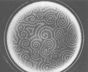
The xyz elements of c represent the populations of vegetation, herbivores, and predators respectively. On a large scale, the dynamics of animal populations generate interesting patterns:
In real life, these kinds of patterns are most easily seen with microbe populations in a petri dish, but the same laws govern large animal populations across the globe.
Humanity
Concluding the prelude on the early earth, the pace slows to a cycle between day and night, terrain becoming fixed as tectonic movements become imperceptible. Soon the night reveals unprecedented patterns of light, as humanity proceeds to colonise the surface of the planet.
This rapid expansion brings its own set of changes, as humans begin to burn large amounts of fossil fuels to power their settlements. Carbon that had lain dormant for millions of years is released into the atmosphere, and dispersed around the planet.
Over several hundred years, humans burn through all available fossil fuel resources, releasing five trillion tonnes of carbon into the atmosphere. This strengthens the greenhouse effect, raising the global average temperature by almost 10 degrees Celsius. Large regions of land around the equator are rendered uninhabitable by extreme temperatures, resulting in the disappearance of humanity from a significant portion of the planet.